Gradient Alignment Test

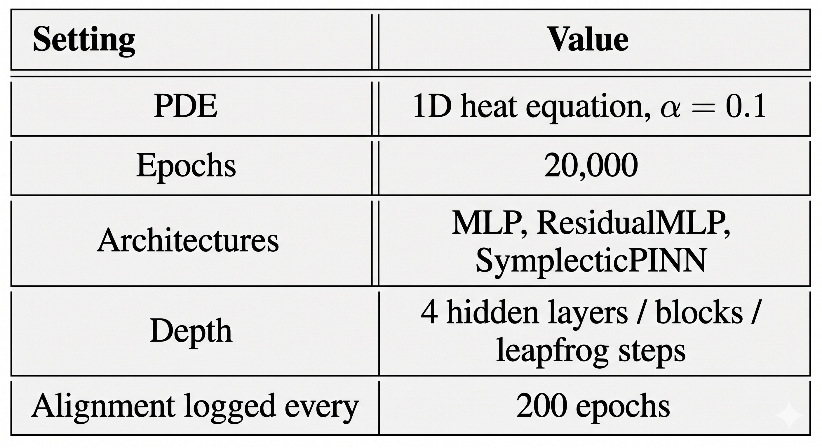
Purpose

This is the primary proof for Goal 3 (Teamwork) — the hypothesis that symplectic structure reduces conflict between the PDE residual loss and the boundary condition loss during training. A standard PINN optimizes both simultaneously, and their gradients can point in opposing directions, creating instability.

The diagnostic directly measures this conflict by computing the cosine similarity between ∇L_pde and ∇L_bc at each training step. A value near −1 means the two objectives are actively fighting each other; a value near +1 means they are aligned.

The multi-objective nature of PINN training is a known source of instability. Abijuru et al.^[5] characterize two key failure modes: gradient shattering, where gradients weaken across depth, and flow mismatch, where optimization directions diverge from the physically meaningful solution trajectory. Gradient alignment is the direct experimental window into flow mismatch: sustained negative cosine similarity is the signal-level manifestation of updates that improve one loss at the cost of another. This experiment runs the measurement under the simplest controlled conditions — a single depth — before Experiment 4 extends it across the depth axis.

Diagnostic methodology

The test computes, at each logged training step:

• ∇L_pde — gradient of the PDE residual loss with respect to all model parameters.
• ∇L_bc — gradient of the boundary condition loss with respect to all model parameters.
• cos(∇L_pde, ∇L_bc) — the cosine similarity of these two gradient vectors, ranging from −1 (perfect conflict) to +1 (perfect alignment).

This is run for all three architectures — MLP, ResidualMLP, and SymplecticPINN — under identical training conditions on the 1D heat equation. The cosine similarity diagnostic is well-established in the multi-task gradient literature as the most direct measure of whether shared parameters can simultaneously serve multiple objectives.

Setup

Results

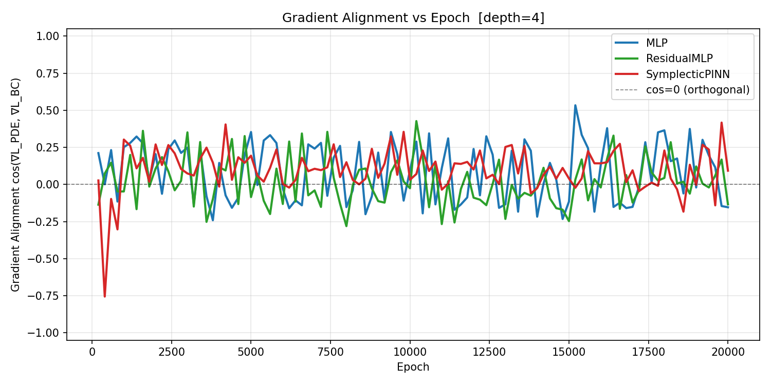
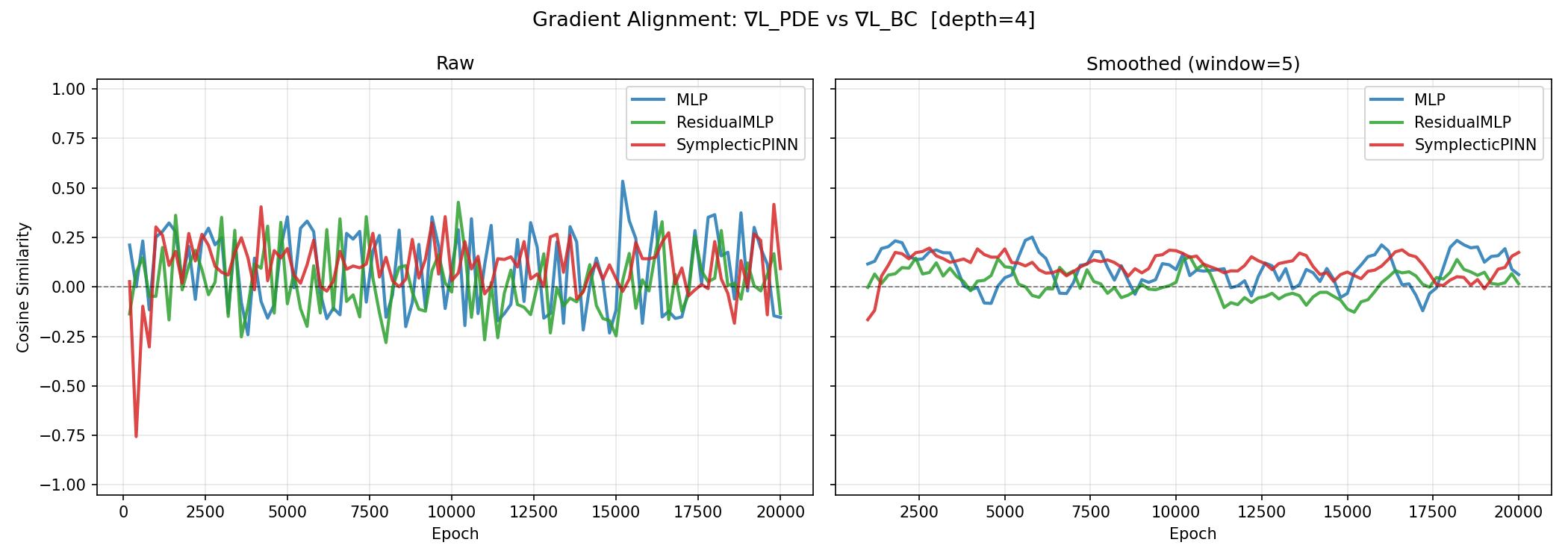
Observations

The SymplecticPINN maintains consistently higher (less negative) gradient alignment throughout training compared to the MLP. The smoothed plot makes the structural difference visible: the MLP alignment fluctuates widely and spends extended periods in negative territory, while the SymplecticPINN alignment is more stable and more frequently positive.

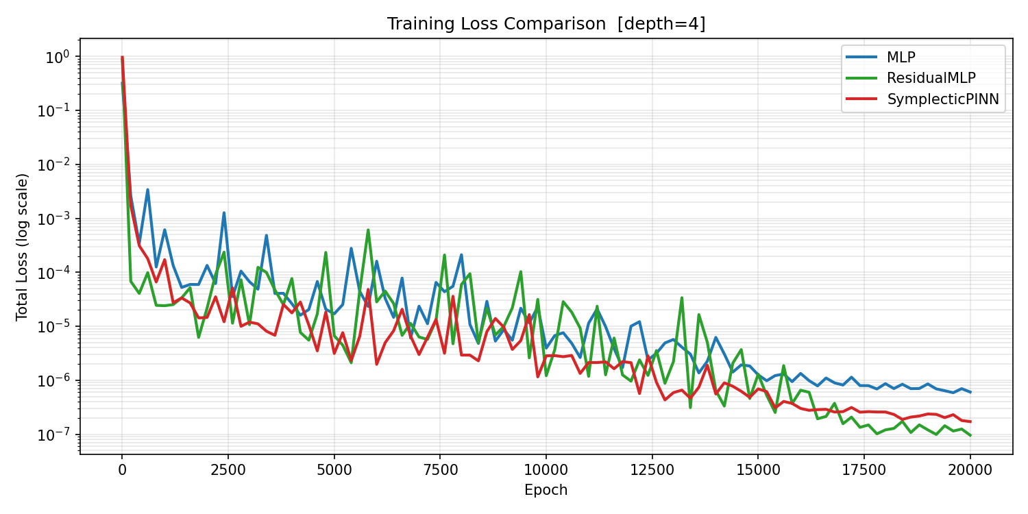
This is consistent with the training spike pattern from Experiment 1. The large loss spikes seen in the MLP curve correspond to epochs where the PDE and boundary gradients are in direct conflict — gradient descent improves one objective at the cost of the other, then must recover. The SymplecticPINN avoids this regime more reliably.

Canizares et al.^[2] show that symplectic neural flows trained on Hamiltonian systems maintain improved energy conservation compared to general-purpose integrators, with backward error analysis providing guaranteed proximity to an exact Hamiltonian flow. In our setting the relevant conserved quantity is not physical energy but gradient coherence across objectives. The Greydanus et al.^[4] result — that Hamiltonian inductive bias enables networks to discover conservation laws without supervision — motivates the expectation that phase-space structure should translate into more cooperative training dynamics, a prediction this experiment confirms empirically.