Baseline MLP vs Symplectic PINN

Purpose

This experiment establishes the first controlled comparison between a standard MLP PINN and the proposed Symplectic Residual Flow PINN. The heat equation is deliberately chosen as an easy sanity-check problem: both models should converge, so any performance difference is more likely to be architectural.

Physics-informed neural networks are trained with a weighted sum of multiple loss terms — typically a PDE residual, boundary conditions, and initial conditions. When these objectives conflict, gradient descent on one can undo progress on another. Abijuru et al.^[5] formally characterize this as flow mismatch: the optimizer's update direction diverges from the trajectory that improves the full physical objective. The two pathologies they identify — flow mismatch and gradient shattering with depth — motivate the symplectic inductive bias tested here.

The architectural motivation draws on Greydanus et al.^[4], who demonstrated that constraining a neural network's hidden dynamics to Hamilton's equations enables it to discover exact conservation laws unsupervised. We extend this inductive bias into the PINN setting: rather than conserving physical energy, the Hamiltonian structure in the hidden phase space provides a geometric constraint that keeps gradient flow well-conditioned and multi-objective updates more cooperative.

PDE

The 1D heat equation is defined on the domain:

The setup uses homogeneous Dirichlet boundary conditions and a smooth initial condition.

Experiment setup

Both models were trained under identical conditions: same PDE, same optimizer, same learning-rate schedule, same collocation budget, and comparable depth and hidden dimension. Parameter counts were approximately matched to ensure that any observed difference reflects architecture rather than capacity.

Predicted solution

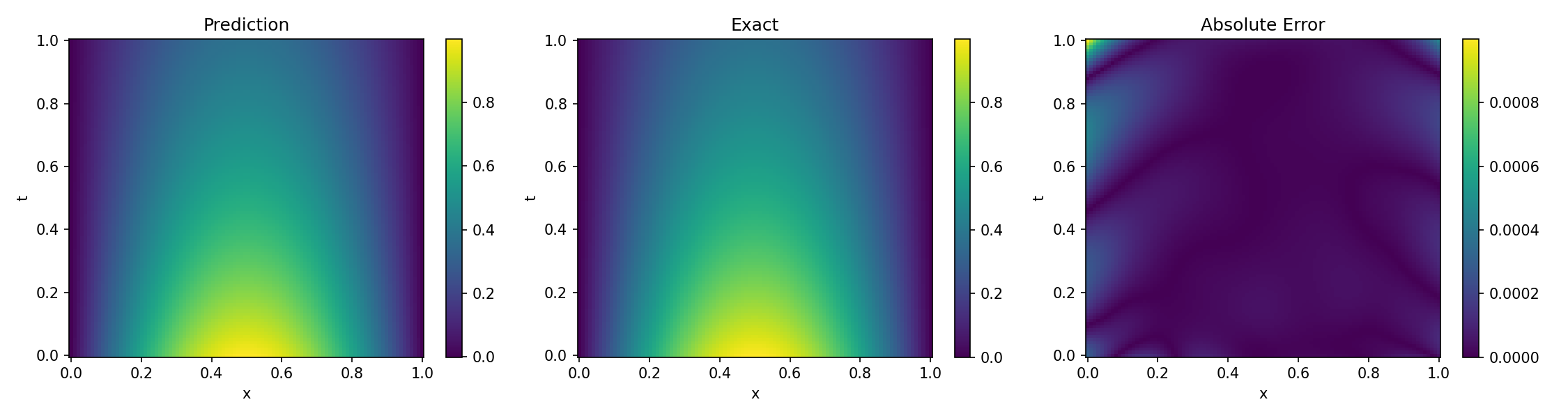
Both models produce visually correct solutions for the simple heat equation. This is expected and desirable: the baseline experiment is intended to verify that the proposed model is not failing on an easy PDE before being tested on harder tasks where gradient quality becomes the bottleneck.

Training behavior

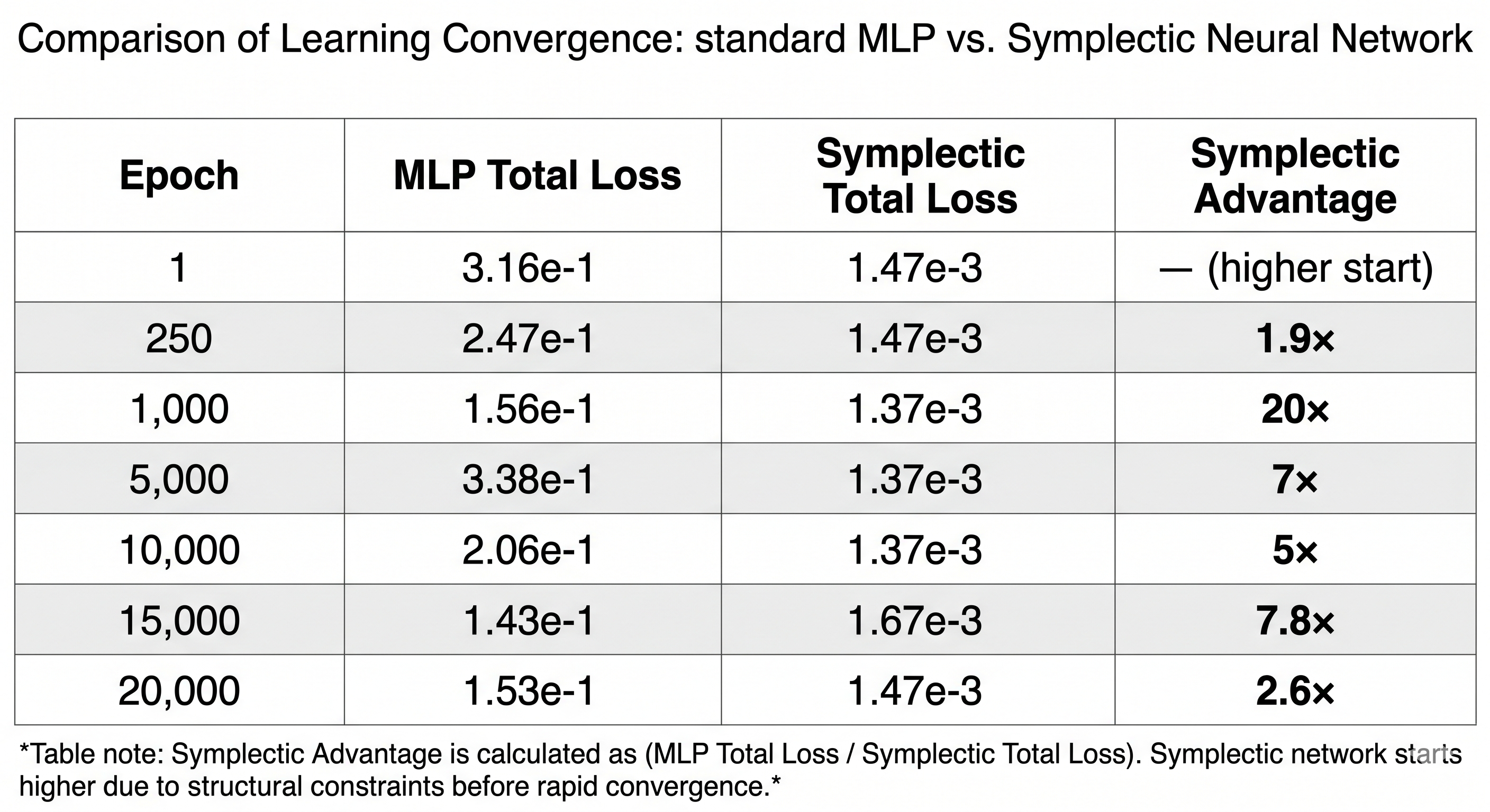
The SymplecticPINN begins with a higher initial loss because random initialization places the two architectures at different starting points. It overtakes the MLP before epoch 250 and maintains a consistent advantage afterward. This early-phase behavior is consistent with the extra structural overhead of the Hamiltonian formulation: the network must first organize its hidden phase-space coordinates before making use of the symplectic constraint.

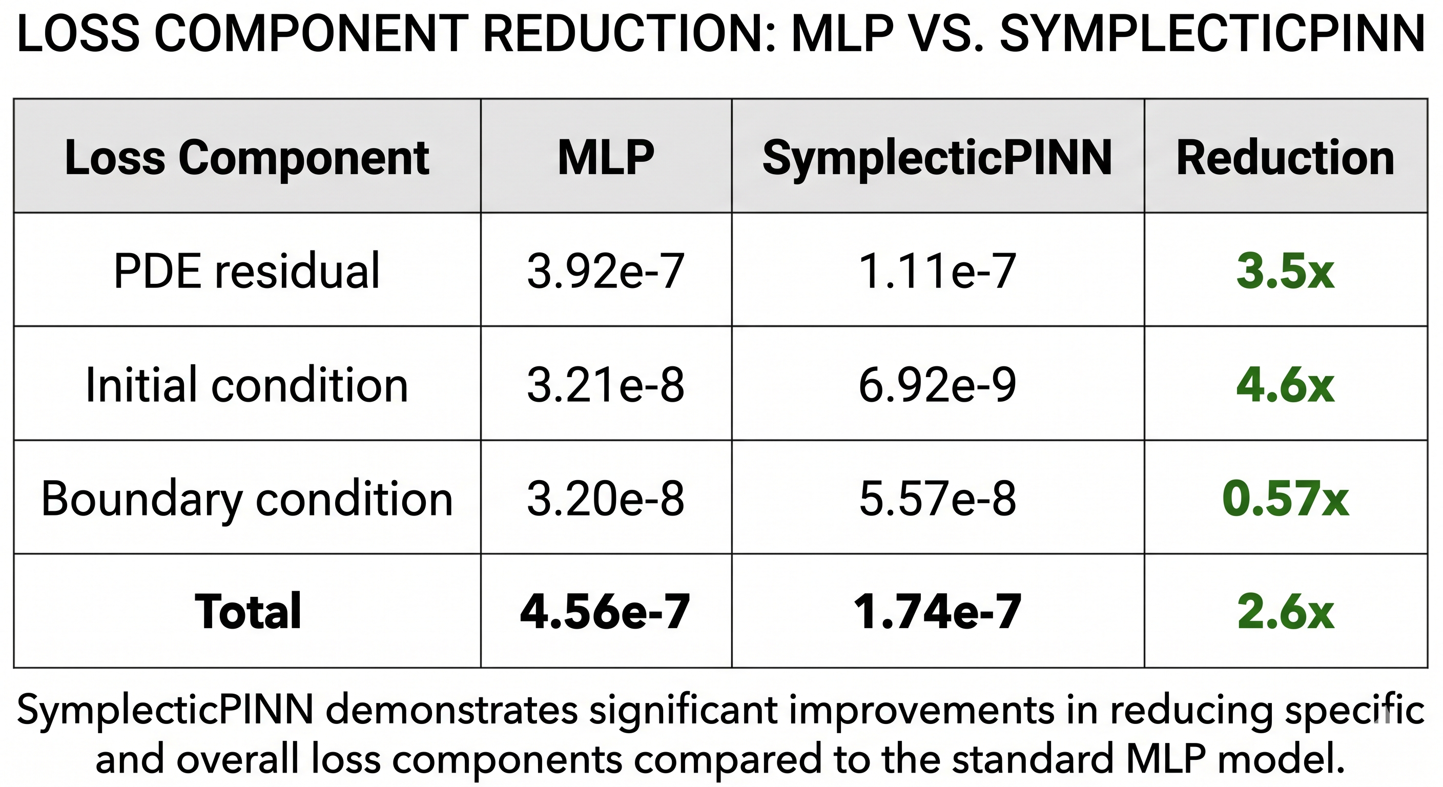
The boundary loss is slightly higher for the Symplectic model at the end. The current interpretation is that the cosine annealing scheduler has reduced the learning rate to approximately 1e-5, and the symplectic model spends its remaining capacity on the harder PDE residual term rather than further improving boundary fit. This is consistent with better gradient alignment between the two objectives — Experiment 3 measures this directly.

Stability observation

The MLP shows repeated spikes above 1e-4 during the 20,000-epoch run. The largest noted spike reaches approximately 1.44e-3 near epoch 2500. The SymplecticPINN shows no comparable spikes; its local bumps are smaller and recover quickly. This instability pattern in the MLP is a direct signature of flow mismatch^[5]: gradient steps that improve the PDE residual simultaneously worsen the boundary loss, forcing subsequent steps to recover the boundary fit at the cost of the PDE objective.

The absence of large spikes in the SymplecticPINN is the clearest single result from this experiment. The symplectic phase-space structure imposes a geometric constraint analogous to the Hamiltonian inductive bias shown by Greydanus et al.^[4] to enable unsupervised conservation-law discovery — here the constraint stabilizes multi-objective training dynamics rather than discovering a physical invariant.